A duplex number is an expression like 5 ± 2 ± 1, read as one number that holds several values at the same time. This page explains the notation, shows what it can represent, and has a calculator so you can try it for yourself.
Normally a ± sign is shorthand for two separate answers. Here it is treated as part of the number.
Write 5 ± 2 and you have a single number with two values, 3 and 7. Add another ± and each of those values splits again. The first number is the centre, and each number after a ± is a spread.
5
5 ± 2
5 ± 2
                        ± 1
5 ± 2
                        ± 1
                        ± 0.5
An expression with n spreads has 2n values, but you only write down n + 1 numbers. The notation stays short while the distribution it describes doubles with every ±. Values can repeat: 5 ± 1 ± 1 gives 3, 5, 5 and 7, so the result is a multiset, and 5 counts twice.
Multiplying two different duplex numbers usually gives values that no duplex number can hold. What happens instead, and how far the notation can be stretched to cover it, is in the panel below.
Every sign of one meets every sign of the other. Sometimes the result is still a duplex number: (0 ± 2)(0 ± 2) is 4, −4, −4, 4, which is 0 ± 4. Usually it is not: (5 ± 2)(3 ± 1) is 6, 12, 14 and 28, and no centre makes those symmetrically spaced.
The fix is a duplextended number, where other operator pairs join ± in the chain. The first is ⋇, multiply-divide: a ⋇ r is a ÷ r and a × r at once. Any single-± number with positive values is also a ⋇ number, 3 ± 1 is √8 ⋇ √2, so a product folds into one ± chain followed by a ⋇ chain:
Four numbers written, four values: 6, 12, 14, 28. The calculator below works this out for any product.
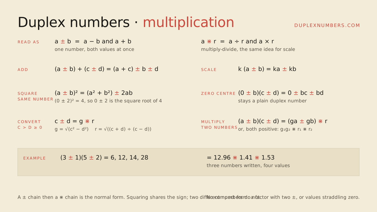
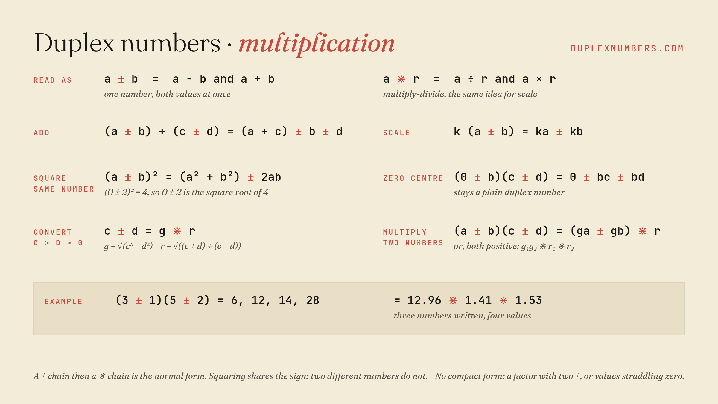
The extended numbers do not close the notation under multiplication. They extend it to cover one more kind of factor, at the cost of one extra number per factor. The rules fit on one card: multiplication.svg, also as a png.
Yes, and it is the values themselves. Write out all 2n values of a duplex number as a list, one per choice of signs. Lists add and multiply entry by entry, and every law of arithmetic holds. That list algebra is the full algebra, and the calculator's resulting distribution is an element of it.
A duplex number is the special case where the list has the form a ± b ± c. For one spread, every list of two values has that form, so the duplex numbers and the full algebra are the same thing, the split-complex numbers, and multiplication with a shared sign stays inside: (5 ± 2)(3 ± 1) = 17 ± 11. In this algebra 0.5 ± 0.5 is a number equal to its own square, and a number with that property, other than 0 and 1, is exactly a number that is 0 in one place and 1 in another. The equality reading in the superposition section is that fact.
For two or more spreads the duplex numbers are a slice of the full algebra, n + 1 numbers out of 2n, and no slice that small can be closed under multiplication: the signs tell every choice apart from every other, and anything closed under multiplication that can tell all the choices apart must be the whole algebra. So there is a choice. Keep the short writing and lose closure, or keep closure and write all 2n numbers. The duplextended form is a chart for a few extra points that the slice misses, and the ⋇ rule is what it costs to reach them.
Build an expression and change the numbers. The tree shows how the values split at each ±, and every leaf is one way of choosing the signs. The distribution lists every leaf, repeats included. Two paths can land on the same value. That does not make two values: 5 is still 5, so the underlying set is the list of numbers the duplex number is equal to, and the distribution records how the signs got there. Tick the box to switch between them.
A duplex number does not just list its values. It says they are the same number.
Take 0.5 ± 0.5.
Its values are 0 and 1, and the duplex number is a way of
writing down that 0 and 1 are equal. In ordinary arithmetic
"1 = 0" is false, and a system that accepts it collapses:
every number becomes equal to every other. A duplex number
accepts the equation anyway, but keeps both sides written as
a centre and a spread, so the collapse stays inside the number
that contains it. That is what this site means by
superposition: a number that is several values and treats
them as one.
Things do break. You cannot ask which value a duplex number has, and multiplying two different duplex numbers usually leaves the duplex form. But a surprising amount still works. You can add them, scale them, take their mean and variance, and read the eigenvalues of a matrix off one. The parallel lines section shows the clearest case: two lines that never meet produce a contradiction, the contradiction becomes a duplex number, and the number draws both lines.
The rule for what still works is this: a duplex number is one number, so it takes one value everywhere it appears in a calculation. Square 0 ± 2 and −2 is paired with −2 and 2 with 2, never −2 with 2. Both paths give 4, so (0 ± 2)² = 4, and 0 ± 2 is the square root of 4, both roots, as one number. The same rule squares the number above: (0.5 ± 0.5)² is 0.5 ± 0.5, its own square, just as 0 and 1 are. Two different duplex numbers do not share a sign, which is why their product behaves differently.
Square it with the shared-sign rule and it comes back unchanged: (0.5 ± 0.5)² = 0.5 ± 0.5. A number that equals its own square, other than 0 and 1, is called an idempotent, and in the two-value algebra of one ± the idempotents are exactly the numbers that are 1 in one place and 0 in the other. Multiply it by its mirror, 0.5 ∓ 0.5, and you get 0, so the algebra splits into two halves along it. Algebraists call this a Peirce decomposition. "A number that is 0 and 1 at once" is the plain-English reading of that theorem, not a figure of speech.
The same number answers a question that has been argued over
since 1703: what is the sum of
1 − 1 + 1 − 1 + 1 − 1 + …? Stop after an even
number of terms and you get 0. Stop after an odd number and you
get 1. Different ways of summing the series give different
answers, and the Cesàro sum, which averages the partial sums,
gives ½. The duplex number
0.5 ± 0.5 holds all
three answers in one expression: a centre of ½, with values 0
and 1.
The values of a duplex number are spaced symmetrically around their centre a, wherever that centre sits on the number line, so the multiset is a distribution and two statistics can be read off without expanding anything. Repeated values count each time they occur.
The centre. Every ± steps the same distance either side of it.
Each spread contributes its square, the same way independent errors add.
Another way to see it: choose each sign by tossing a coin. Then a duplex number is a random walk that starts at a and steps b to the left or right, then c, and so on. Probability theory calls the total a Rademacher sum, and its mean and variance are exactly the ones above.
The reverse only goes so far. Symmetric here means spaced evenly about some centre, not about zero. Any pair of values is a duplex number, its centre being their midpoint, and so is any four values that mirror about their midpoint, because the two gaps fix b and c. From eight values upward there are more points than coefficients, so most symmetrically spaced sets have no duplex form.
If the chain never stops, take 0 ± 1 ± λ ± λ² ± … for some λ between ½ and 1. The limit is called a Bernoulli convolution. Which values of λ give a smooth distribution is a question Erdős raised in 1939, and it is still open.
The quadratic formula gives the eigenvalues of a 2×2 matrix in ± form already, so both fit in one duplex number. Type numbers into the matrix to see it.
Write the diagonal as a ± b and the off-diagonal
as c ± d. When b = d the eigenvalues are simply
a ± c. Otherwise they are
a ± √(b² + c² − d²).
A duplex number is also a matrix in its own right. Put the centre on every diagonal entry, then add the spread to one entry and subtract it from the other. The result has the two values of the duplex number on its diagonal, and a diagonal matrix has its diagonal as its eigenvalues.
Each further ± doubles the size of the matrix. The first spread is added to the top half and subtracted from the bottom half, the second alternates entry by entry, and so on. The diagonal is the calculator's tree, read from the leftmost leaf to the rightmost.
5 + 2 + 1, 5 + 2 − 1, 5 − 2 + 1, 5 − 2 − 1. A repeated path is a value that appears twice on the diagonal.
The 2×2 formula above extends to any matrix built from independent parts. Find the duplex number of each part with the formula, then add the duplex numbers. The combined matrix is full of off-diagonal entries, but its eigenvalues are still one chain.
The combined matrix applies part 1 to the first half of each state and part 2 to the second half, and each combination of one eigenvalue from each part appears once. That is duplex addition: the four eigenvalues are 1, 4, 5 and 8.
Physicists meet this every day. A system made of n independent parts, each of which can be in one of two states, has 2n energy levels, and they are always a duplex number: E₀ ± ε₁ ± ε₂ ± … The n spreads come from a problem of size n, not 2n, which is why such systems are called exactly solvable. Levels that coincide are repeated paths. When the parts interact, extra terms appear that the notation cannot hold, in the same way that multiplying two duplex numbers leaves the duplex form.
Take two parallel lines, y = x + 1 and
y = x + 3, and ask where they cross. Set them
equal and the x cancels, leaving 1 = 3. In
ordinary algebra that contradiction is the end of the story:
there is no solution, so the lines never meet.
Now do what the superposition section did with 1 = 0. Read the
contradiction as a duplex number: 1 and 3 together are
2 ± 1. Put that
back into the equation and you get
y = x + (2 ± 1),
one equation whose graph is both lines. The contradiction has
not been thrown away. It has become the spread.
The plot below draws
y = (m ± k)x + (b
                ± d)
. With no slope
spread it is a family of parallel lines. Give the slope a
spread as well and a choice appears: are the two
± signs the same sign, or
independent? Independent signs give four lines. A shared sign
gives two, with the steeper slope paired to the higher
intercept, because one sign choice picks both. The rule from
the superposition section decides which you get. Build the
slope and intercept from one duplex number, t = 0
± 1, as
y = (m + kt)x + (b + dt), and t takes one value
in both places, so there are two lines. Write them as two
separate duplex numbers and the signs are independent, so
there are four. A plain set of values cannot express that
difference. It only records which values occur.
Duplex numbers can help build an intuition for what a quantum computer does. Think of a duplex number as an extra numerical type available on the machine, one that can take a modulus or raise to a power across every value it holds in a single operation. On an ordinary computer each value would have to be handled separately, and the work grows with the number of values represented, which for a chain of n spreads is 2n.
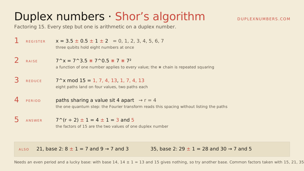
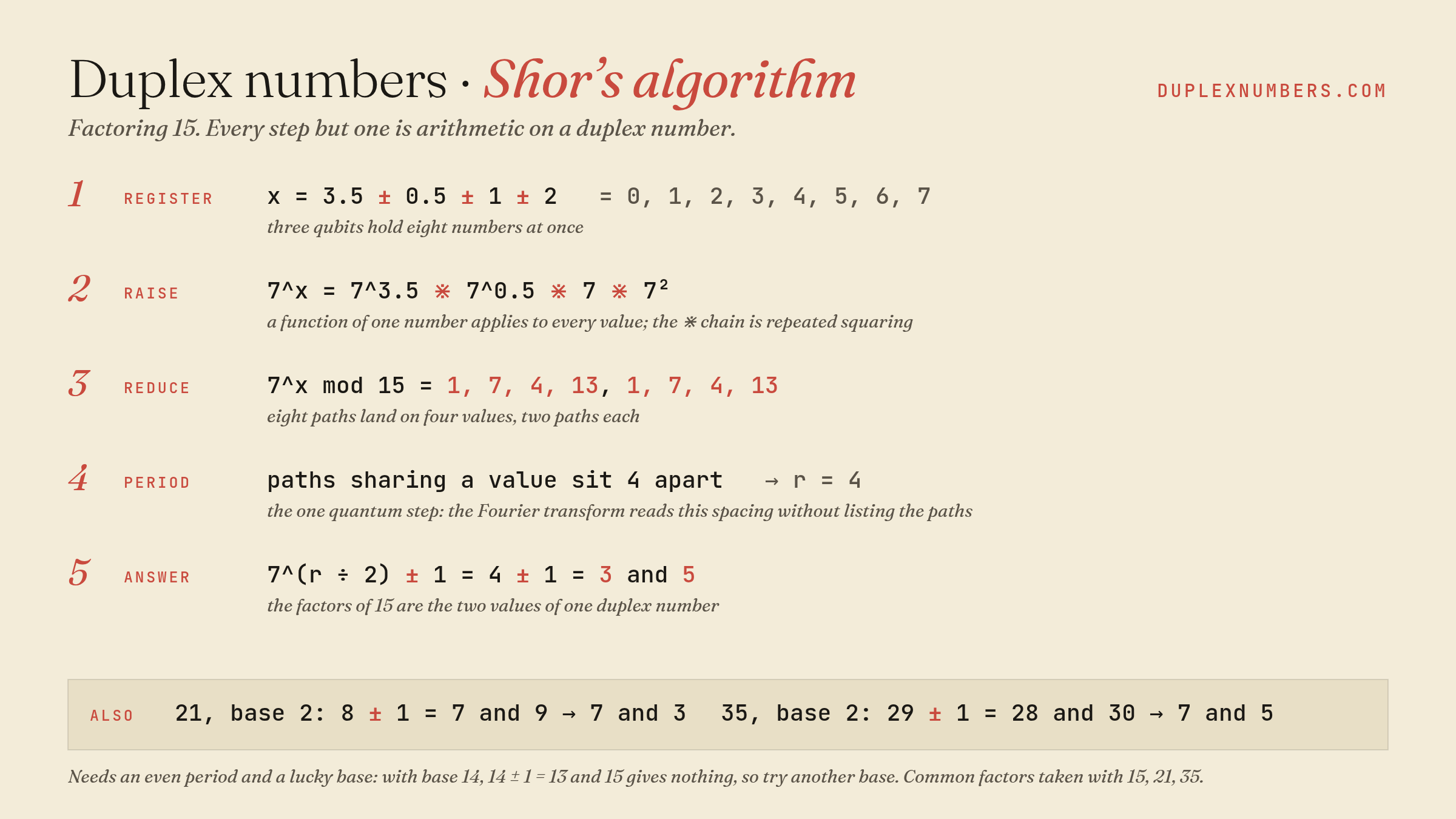
The clearest example is Shor's algorithm for factoring. The register is a duplex number, raising a base to it is a function applied value by value, the period of the result shows up as repeated paths, and the final step, ar/2 ± 1, is a duplex number whose two values are the two factors. The one step that needs the quantum computer is reading the period without listing the paths. The walk-through for 15 fits on one card: shor.svg, also as a png.
Found a new use for duplex numbers? Open a pull request.